The Law of Total Variance Is Counterintuitive

The law of total variance states that for two random variables \(X\) and \(Y\),

\[\mathrm{Var}(Y) = E[\mathrm{Var}(Y | X)] + \mathrm{Var}(E[Y | X])\]

If \(Y\) is a mixture of distributions, this tells you that \(\mathrm{Var}(Y)\) is the mean variance of the components plus the variance of the means of the components (\(X\) in this case is a discrete variable indicating which component you selected).

At first blush this makes sense: jumping from \(\bar{Y}\) to \(\mu_i\) (the mean of component \(i\)) gives you some variance, and then jumping from \(\mu_i\) to your sample gives you some additional variance. But! These are dependent jumps, so you can’t naively add the variances.

Some pretty graphs

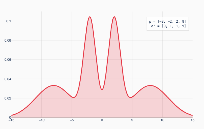
Let’s concretely say we have an equal mixture of 4 Gaussians with means -8, -2, 2, and 8. If the 2 outer Gaussians have variance 9 and the inner Gaussians have variance 1, you get this distribution:

Compare this to a version where the inner Gaussians have high variance:

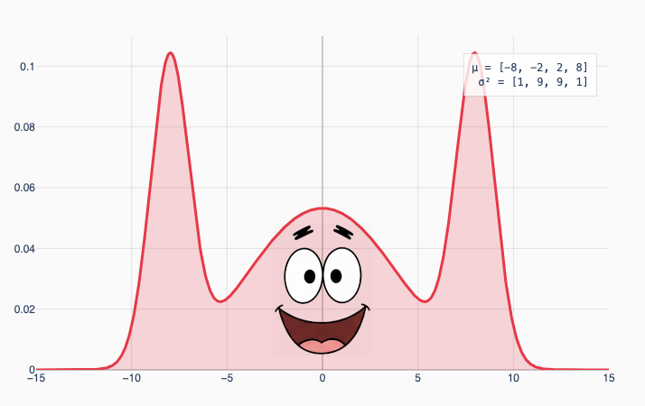
The law of total variance says these two distributions have exactly the same overall variance (which works out to 39). That’s surprising to me! I would intuitively expect the first graph to have higher variance because the wider Gaussians on the edges lead to more extreme values.

A discrete version

Let’s try to understand what’s happening by replacing these Gaussians with Bernoulli distributions ¹ with the same means and variances. For example, a Gaussian with mean 2 and variance 9 becomes a coin flip where heads is 5 and tails is -1.

	scenario 1		scenario 2
$$\mu_i$$	$$\sigma_i$$	samples	$$\sigma_i$$	samples
-8	3	-11, -5	1	-9, -7
-2	1	-3, -1	3	-5, 1
2	1	1, 3	3	-1, 5
8	3	5, 11	1	7, 9

The variances of the two lists [-11, -5, -3, -1, 1, 3, 5, 11] and [-9, -7, -5, -1, 1, 5, 7, 9] are indeed both 39. Cool I guess? But it’s not really illuminating.

Instead let’s sic ✨algebra✨ on the problem. We’ll zoom in on one of these Bernoulli distributions which is a coin flip between \(\mu_i - \sigma_i\) and \(\mu_i + \sigma_i\). We can add up their contributions to the variance. (Here \(N=8\) is the total number of samples):

\[\frac{(\mu_i - \sigma_i)^2}{N} + \frac{(\mu_i + \sigma_i)^2}{N} = 2\frac{\mu_i^2 + \sigma_i^2}{N}\]

So on average, each sample contributes \(\frac{\mu_i^2 + \sigma_i^2}{N}\) to the total variance. That’s what the law of total variance says! It works, at least in this simple case.

OK so why does it actually work

\(\mathrm{Var}(X + Y) = \mathrm{Var}(X) + \mathrm{Var}(Y)\) if \(X\) and \(Y\) are uncorrelated. They don’t necessarily need to be independent (which is a stronger condition). You can see this from the more general formula

\[\mathrm{Var}(X + Y) = \mathrm{Var}(X) + \mathrm{Var}(Y) + 2\mathrm{Cov}(X, Y)\]

which works for all \(X\) and \(Y\). Here, once we pick \(X=\mu_i\), the distribution of \((Y \vert X = \mu_i) - \mu_i\) is zero-mean by definition, and so it’s uncorrelated with which \(\mu_i\) we chose.